单细胞相关分析技能
1.批次效应去除
1.1 方法文献
Korsunsky, I., Millard, N., Fan, J. et al. Fast, sensitive and accurate integration of single-cell data with Harmony. Nat Methods 16, 1289–1296 (2019). https://doi.org/10.1038/s41592-019-0619-0
1.2 使用案例
https://github.com/immunogenomics/harmony
(1) 加载案例数据,并构建Seurat对象
pbmc.stim, pbmc.ctrl是2给批次的单细胞数据。
library(Seurat)
data("pbmc_stim")
pbmc <- CreateSeuratObject(counts = cbind(pbmc.stim, pbmc.ctrl),
                           project = "PBMC", min.cells = 5)
(2) 添加批次信息
## Separate conditions
pbmc@meta.data$batch <- c(rep("STIM", ncol(pbmc.stim)), rep("CTRL", ncol(pbmc.ctrl)))
(3) 数据的归一化
pbmc <- pbmc %>%
  NormalizeData(verbose = FALSE)
VariableFeatures(pbmc) <- split(row.names(pbmc@meta.data), pbmc@meta.data$batch) %>% lapply(function(cells_use) {
  pbmc[,cells_use] %>%
    FindVariableFeatures(selection.method = "vst", nfeatures = 2000) %>%
    VariableFeatures()
}) %>% unlist %>% unique
(4) PCA降维
pbmc <- pbmc %>%
  ScaleData(verbose = FALSE) %>%
  RunPCA(features = VariableFeatures(pbmc), npcs = 20, verbose = FALSE)
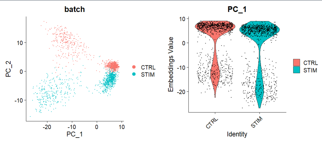
(5) 去除批次效应前的可视化
## 未进行批次效应校正
library(cowplot)
options(repr.plot.height = 5, repr.plot.width = 12)
p1 <- DimPlot(object = pbmc, reduction = "pca", pt.size = .1, group.by = "batch")
p2 <- VlnPlot(object = pbmc, features = "PC_1", group.by = "batch", pt.size = .1)
plot_grid(p1,p2)
(6) 运行RunHarmony去除批次效应
bacth就是分组变量,相当于2个批次效应的单细胞数据分组信息pbmc@meta.data$bacth。
pbmc <- pbmc %>%
  RunHarmony("batch", plot_convergence = TRUE,
             nclust = 50, max_iter = 10, early_stop = T)
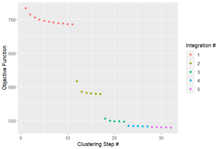
通过设置plot_converge=TRUE,Harmony将生成一个显示整合流程的目标图。每个点代表经过一轮聚类后测量的成本。不同的颜色代表由max_iter控制的不同Harmony迭代(假设early_stop=FALSE)。这里max_iter=10,预期最多有10个修正步骤。然而,由于early_stop=TRUE,Harmony将在成本达到稳定后停止。
RunHarmony函数中主要参数:
group.by.vars:
- 参数类型:字符向量(character vector)
- 描述:该参数用于指定按照哪些变量对数据进行分组,以便进行整合。
- 示例:如果数据集包含批次信息和其他变量,可以将批次信息放在一个变量中,并将该变量传递给group.by.vars参数,以便根据批次信息对数据进行整合。
max.iter.harmony:
- 参数类型:数值型(numeric)
- 描述:设置Harmony算法的最大迭代次数。默认值为10。
- 示例:如果您希望算法运行更多或更少的迭代次数,可以调整此参数的值。
lambda:
- 参数类型:数值型(numeric)
- 默认值:1
- 描述:决定了Harmony整合的力度。lambda值越小,整合力度越大;反之,lambda值越大,整合力度越小。调整范围一般在0.5-2之间。
- 示例:如果您希望增强整合力度,可以将lambda值调小;如果您希望减小整合力度,可以将lambda值调大。
theta:
- 参数类型:数值型(numeric)
- 描述:Diversity clustering penalty parameter。为group.by.vars中的每个变量指定。默认theta=2。theta=0不鼓励多样性。较大的theta值导致更多样化的集群。
- 示例:根据您的数据和研究目的,可以调整theta的值以获得不同的聚类效果。
dims.use:
- 参数类型:数值型向量(numeric vector)或字符型向量(character vector)
- 描述:指定用于Harmony的PCA维度。默认情况下,使用所有PCA维度。
- 示例:如果您只对PCA的前几个维度感兴趣,可以将dims.use参数设置为一个数值向量,例如dims.use = c(1, 2)。
sigma:
参数类型:数值型(numeric)
- 默认值:0.1
- 描述:软k均值聚类的宽度。它决定了从单个细胞到聚类中心的距离。较大的sigma值导致细胞被分配到更多的聚类中,而较小的sigma值使软k均值聚类接近于硬聚类。
- 示例:根据您的数据和聚类需求,可以调整sigma的值以获得不同的聚类效果。
这些参数共同决定了Harmony算法在运行时的行为和结果。根据您的具体需求和数据特征,您可能需要调整这些参数以获得最佳的分析效果。在使用Harmony包时,请确保仔细阅读相关文档和教程,以便更好地理解这些参数的作用和最佳实践方法。
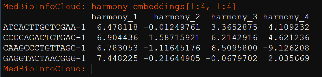
RunHarmony的运行结果在pbmc@reductions$harmony中。
使用Embeddings命令访问新的Harmony embeddings。
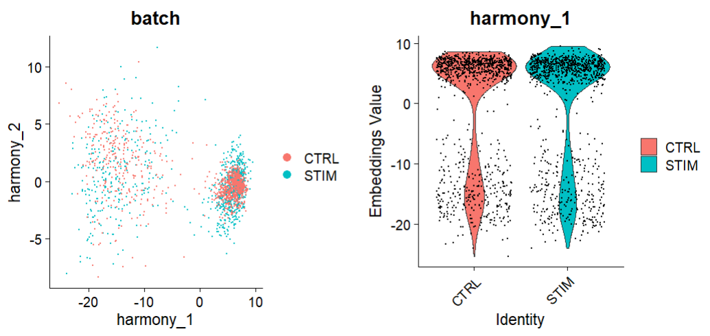
(7) 去除批次效应后的可视化
options(repr.plot.height = 5, repr.plot.width = 12)
p1 <- DimPlot(object = pbmc, reduction = "harmony", pt.size = .1,
              group.by = "batch")
p2 <- VlnPlot(object = pbmc, features = "harmony_1",
              group.by = "batch", pt.size = .1)
plot_grid(p1,p2)
1.3 参考资料
https://github.com/immunogenomics/harmony
https://htmlpreview.github.io/?https://github.com/immunogenomics/harmony/blob/master/doc/Seurat.html
2.CopyKAT——恶性和非恶性上皮细胞的识别
2.1 方法文献
Gao, R., Bai, S., Henderson, Y.C. et al. Delineating copy number and clonal substructure in human tumors from single-cell transcriptomes. Nat Biotechnol 39, 599–608 (2021). ttps://doi.org/10.1038/s41587-020-00795-2
2.2 使用案例
(1) 包的安装
(2) 读入单细胞数据
单细胞数据的两种读入方式

library(Seurat)
library(copykat)
dirpath = "H:/DatabaseData/scRNAseq/BRCA"
raw <- Read10X(dirpath)
raw <- CreateSeuratObject(counts = raw, project = "copycat.test", min.cells = 0, min.features = 0)
exp.rawdata <- as.matrix(raw@assays$RNA@counts)
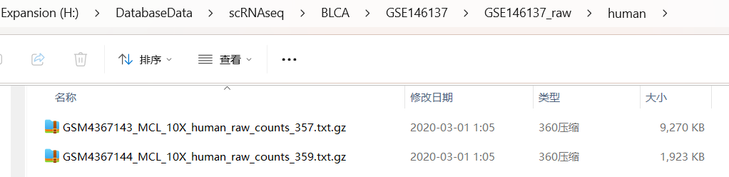
folder = "H:/DatabaseData/scRNAseq/BLCA/GSE146137/GSE146137_raw/human"
samples=list.files(folder)
samples
# pro <- samples[1]

sceList = lapply(samples,function(pro){
  folder= file.path(folder,pro)
  raw.data <- read.table(folder,sep = "\t",header = T,
                         row.names = 1,check.names = F)
  CreateSeuratObject(counts = raw.data,
                     project = unlist(strsplit(pro,"_"))[1] )
})
sce.big <- merge(sceList[[1]],
                 y = c(sceList[[2]]),
                 add.cell.ids = samples,
                 project = "GSE146137")
exp.rawdata <- as.matrix(sce.big@assays$RNA@counts)
(3) 执行copykat
library(copykat)
copykat.test <- copykat(rawmat=exp.rawdata, id.type="S",
                        ngene.chr=5, win.size=25, KS.cut=0.1,
                        sam.name="test", distance="euclidean",
                        norm.cell.names="",
                        output.seg="FLASE", plot.genes="TRUE",
                        genome="hg20",n.cores=1)
Cellranger输出的默认基因ID是基因符号,所以id.type为“Symbol”或“S”。为了过滤细胞,ngene.chr要求每个染色体中至少有5个基因来计算DNA拷贝数。可以将其调低为ngene.chr=1以保留尽可能多的细胞,但使用少于5个基因来代表一个染色体并不是很严格。为了过滤基因,我可以调整参数只保留在LOW.DR到UP.DR细胞分数中表达的基因。我设置默认的LOW.DR=0.05,UP.DR=0.2。我可以调低这些值以在分析中保留更多的基因。不过我需要确保LOW.DR小于UP.DR。
要求copykat每个片段至少取25个基因。我可以尝试其他选项,每个bin的范围是15-150个基因。KS.cut是分割参数,范围从0到1。增加KS.cut会降低敏感性,即减少片段/断点。通常它的工作范围是0.05-0.15。
在这里,我通过设置n.cores = 4进行并行计算。默认值是1。
我还通过设置sam.name="test"给出了一个样本名称。
pred.test <- data.frame(copykat.test$prediction)
pred.test <- pred.test[-which(pred.test$copykat.pred=="not.defined"),]  ##remove undefined cells
CNA.test <- data.frame(copykat.test$CNAmat)
预测的结果正常细胞(diploid)还是肿瘤细胞(aneuploid),每个CNV segment在每个细胞的表达量。
(4) navigate prediction results
  my_palette <- colorRampPalette(rev(RColorBrewer::brewer.pal(n = 3, name = "RdBu")))(n = 999)

  chr <- as.numeric(CNA.test$chrom) %% 2+1
  rbPal1 <- colorRampPalette(c('black','grey'))
  CHR <- rbPal1(2)[as.numeric(chr)]
  chr1 <- cbind(CHR,CHR)

  rbPal5 <- colorRampPalette(RColorBrewer::brewer.pal(n = 8, name = "Dark2")[2:1])
  com.preN <- pred.test$copykat.pred
  pred <- rbPal5(2)[as.numeric(factor(com.preN))]

  cells <- rbind(pred,pred)
  col_breaks = c(seq(-1,-0.4,length=50),seq(-0.4,-0.2,length=150),seq(-0.2,0.2,length=600),seq(0.2,0.4,length=150),seq(0.4, 1,length=50))

heatmap.3(t(CNA.test[,4:ncol(CNA.test)]),dendrogram="r", distfun = function(x) parallelDist::parDist(x,threads =4, method = "euclidean"), hclustfun = function(x) hclust(x, method="ward.D2"),
            ColSideColors=chr1,RowSideColors=cells,Colv=NA, Rowv=TRUE,
            notecol="black",col=my_palette,breaks=col_breaks, key=TRUE,
            keysize=1, density.info="none", trace="none",
            cexRow=0.1,cexCol=0.1,cex.main=1,cex.lab=0.1,
            symm=F,symkey=F,symbreaks=T,cex=1, cex.main=4, margins=c(10,10))

  legend("topright", paste("pred.",names(table(com.preN)),sep=""), pch=15,col=RColorBrewer::brewer.pal(n = 8, name = "Dark2")[2:1], cex=0.6, bty="n")
(5) define subpopulations of aneuploid tumor cells
tumor.cells <- pred.test$cell.names[which(pred.test$copykat.pred=="aneuploid")]
tumor.mat <- CNA.test[, which(colnames(CNA.test) %in% tumor.cells)]
hcc <- hclust(parallelDist::parDist(t(tumor.mat),threads =4, method = "euclidean"), method = "ward.D2")
hc.umap <- cutree(hcc,2)

rbPal6 <- colorRampPalette(RColorBrewer::brewer.pal(n = 8, name = "Dark2")[3:4])
subpop <- rbPal6(2)[as.numeric(factor(hc.umap))]
cells <- rbind(subpop,subpop)

heatmap.3(t(tumor.mat),dendrogram="r", distfun = function(x) parallelDist::parDist(x,threads =4, method = "euclidean"), hclustfun = function(x) hclust(x, method="ward.D2"),
            ColSideColors=chr1,RowSideColors=cells,Colv=NA, Rowv=TRUE,
            notecol="black",col=my_palette,breaks=col_breaks, key=TRUE,
            keysize=1, density.info="none", trace="none",
            cexRow=0.1,cexCol=0.1,cex.main=1,cex.lab=0.1,
            symm=F,symkey=F,symbreaks=T,cex=1, cex.main=4, margins=c(10,10))

  legend("topright", c("c1","c2"), pch=15,col=RColorBrewer::brewer.pal(n = 8, name = "Dark2")[3:4], cex=0.9, bty='n')
2.3 参考资料
https://github.com/navinlabcode/copykat
更新: 2023-12-23 15:05:12 原文: https://www.yuque.com/doublehelix/bioinfonotes/snlx1hu2cnsir1dh